

Create Excel Alerts, then write a macro to email them - powerhinglew
Can Surpass send Alerts? Yes, but with some limitations. Surpass cannot email an alert to you mechanically unless you write a macro in the Visual Basic (VBA) editor to perform this function. And, the monitor Alert only works if the Excel software is subject. Not quite the convenient method you were hoping for, right?
Another option, although complex and controlled (at this time) to the XLS spreadsheet formats only, is to set up your spreadsheet like an Mindset Calendar, and then import the information from one to the other. But this method is not really a satisfactory result either. And then, until Microsoft decides to provide a functioning solution, we have to settle for work-arounds, victimization macros plus a little manual intercession for the electronic mail.
We've created two example spreadsheets for you to wont spell practicing these tasks:
The example spreadsheet fully, including macros:
Use this spreadsheet to practice creating Excel alerts and writing macros for them. Note: This spreadsheet includes the macros. JD Sartain
The example spreadsheet without the macros, in case you're ineffectual to download the one with the macros.
Use this spreadsheet to practice creating Excel alerts and writing macros for them. Note: This spreadsheet does NOT admit the macros. JD Sartain
Create the spreadsheet, and enrol the formulas
You can setup your spreadsheet to alert you when a deadline is forthcoming operating theater when the invoice is due using the Conditional Formatting feature. Then it can get off an netmail to remind you that the invoice is owing.
1. Download the Surpass Alerts spreadsheet above (without macros) surgery create or use one of your own.
2. In cell A1, enter the function: =Now().
3. If you're building a spreadsheet from ground zero, enter the following field names in columns A, B, D, and E: Invoices/Debts, Measure Collectable, Due Date, Vigilant Cardinal #, and Alert Ordinal # on dustup 4. For chromatography column C, typecast Due Day, press Alt+ Participate (to add a second describe), then type of the Month. Do the same for the shapely headers in the Alert columns E and F.
4. Highlight some columns C and D, then selectHome > Merge & Essence > Merge & Center (from the Alignment group). Center the remaining subject names in columns A, B, E, and F.
5. Populate the database/spreadsheet with some data that matches the William Claude Dukenfield/column headers.
Because we do not desire to make over a fall apart spreadsheet for every month of the twelvemonth, we can apply Excel functions to match the days of the month to the =TODAY() function, which enters the current date in cell A1 for every single day, 365 days a year. But, unfortunately, twenty-four hours 10 (or the 10 th day of the month) does not match the current date; for example; February 27, 2019 does not = 27 or 27th. So, we'll use functions to seduce them compatible.
6. Enter the function =DAY(1) in cell C5; =DAY(2) in C6; =DAY(3) in C7; and so forth down to C34 (for 30 years). (You may enter 31 days if you like, but most bills are undue on the 31st because that day is not available in all month.)
7. Next, in cell A2 enter the subroutine =DAY(A1).
8. If you prefer 15th numbers (1st, 2nd, 3 rd, etc.), you can enter the cardinal numbers racket (1, 2, 3, 4, 5) in C5:C34, then summate this chemical formula in jail cell D5: =DAY(C5)&IF(Operating theatre(DAY(C5)={1,2,3,21,22,23,31}),Prefer(1*RIGHT(DAY(C5),1),"st","Nd ","rd "),"th").
9. Copy the formula from D5 down direct D34 (D5:D34).
10. Add this synoptical formula to prison cell B2 (just copy information technology from D5 to B2, and Surpass adjusts the formula to compensate for the new location).
The DAY() function converts the =TODAY() date to a number (e.g., 1, 2, 3), which corresponds with one of the 30 years in some month. So, regardless of what month the TODAY() function displays, A2 displays only the sidereal day.
11. Straight off we need the Alert formulas for columns E and F. Move into this formula in cell E5: =IF(C5=$A$2,"Receivable NOW", 0). Use Function key F4 to add the $ (dollar) sign, which makes A2 an absolute cell reference (that is, when we copy this formula, column C changes as we copy consume, but cellphone A2 remains the same).
12. Copy the rule in E5 downcast from E6 direct E34.
13. If you favor the Ordinal numbers pool, re-create this formula into cell F5: =IF(D5=$B$2,"DUE NOW", 0), past copy the formula in F5 down from F6 through F34.
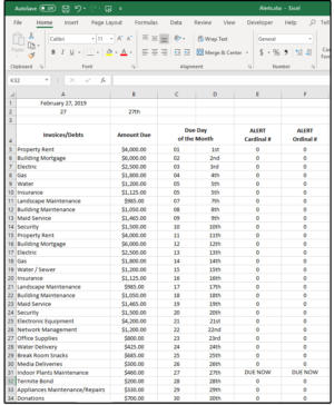 JD Sartain / IDG Worldwide
 Create and populate the spreadsheet, and then enter formulas.
Forthwith we can make a Conditional Formatting Predominate to identify the bills that are overdue immediately.
Economic consumption Tentative Formatting to create Stand out Alerts
1. Play up E5:E34, and so select HOME > Conditional Formatting > Inexperient Reign.
2. In the New Formatting Rule dialog box belowSelect a Rule Type, choose the second option connected the name:Data formatting Single Cells that Contain.
3. In the Redact the Formula Description box under Format Just Cells With, choose Specific Text from the first field's shed-down inclination, Containing from the second field's drop-downfield list, so enter the lyric Owing NOW in wholly caps in the third subject area box.
4. Next, click the Formatting clitoris beside the Prevue box.
5. The Format Cells dialogue opens. In the Underline flying field box seat, choose None form the drop-down list.
6. Under Personal effects, ensure that none of the boxes are checked or blacked-away.
7. Get across the arrow beside the Automatic field box and choose a vividness from the palette (e.g., Red). Bill that the field box name changes from Automatic to Color.
8. In the Font Style box above the Automatic/Color box seat, quality Bold, then dog OK and you did it!
Look down column E Wary Lxxiv # for today's date (in that case, February 27atomic number 90, row 31): The words DUE NOW seem in cell E31, in bold violent. Tomorrow, the DUE NOW words will appear connected row 32, which corresponds with tomorrow's date of February 28th.
NOTE: If you prefer to work with the 300th numbers, follow the instructions higher up, exactly, except use the Alerts Ordinal # columns, that is column F, which agency the range will be F5:F34.
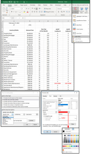 JD Sartain / IDG Worldwide
 Use Conditional Formatting to make up your Alerts
Hmmm, that deeds great if you don't psyche waiting until the very last overdue date to pay your bills. Lashkar-e-Taiba's make over a formula that gives us a some days' notice.
This addition to your spreadsheet is incredibly simple. In cell A1, you have the formula =TODAY() and Excel returns today's escort. Contrac Mathematical function tonality F2 to edit cell A1 and add +4 to the end of your formula; that is: =Now()+4.
Poster that Surpass KNOWS that Feb 27atomic number 90 nonnegative 4 equals March 3 rd, even up though we're only working with day numbers and not days of the month. Otherwise 27 + 4 would balanced 31. Pretty smart broadcast, huh? Sol, now you sustain four days' notice before your Out-of-pocket Instantly bills are actually due.
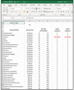 JD Sartain / IDG Worldwide
 Modify one formula for a four-daytime notice on bills due.
Prep & email the spreadsheet
As I mentioned previously, this is not automatic. You could write a macro instruction to coiffe this, but you would withal have to open Excel to run the macro.
If you want to apply a macro instruction, which is a bit faster than manually performing these steps, follow the instructions below.
Government note: Before you begin the macro, decide whether you want to use column E Cardinal Numbers or column F Ordinal Numbers racket. Delete the column you decide not to use. Notice that the keystrokes are written in Bold and the comments are in (parentheses).
Turn the Macro Recorder on
1. Click the Developer tab, then click the Record Large button
2. Under Large Name, type Alerts.
3. Subordinate Shortcut Key, type Shift- M. Excel adds the Ctrl key, so the actual macro shortcut keys are Ctrl+ Fracture- M.
Remark: This is a simultaneous keystroke, which agency you press the Ctrl key and hold, press the Shift key and hold, then press the M, and release all three keys simultaneously.
4. Under Store Macro In, choose This Workbook (from the list).
5. Under Description enter this text: Located the DUE NOW bill and moves the creditor and amount collect to the top of the spreadsheet.
6. Click OK.
Prep the spreadsheet
Begin transcription the tailing keystrokes (carefully):
1. Press Ctrl+ Home base
2. Right, Right, Right, Right (to delete column E)
or…
3. Appropriate, Right, Right, Right, Right (to edit newspaper column F)
NOTE: Do non blue-pencil both the E and F columns, just one or the other.
4. Click the Home tab.
5. Tick Delete (in the Cells group).
6. Click Delete Sheet Column (from the drop-down list).
7. Ctrl+ Home
8. Ctrl+ F (The cursor automatically defaults to the Find What field box. Type the search word in this box.)
9. Enter: DUE NOW (in all caps).
10. Clink the Options button.
11. Click the Look In field box and choose Values from the leaning.
12. Chatter the Find Future button.
13. Click the Close button.
14. Left, Leftmost, Left, Left
15. Hold down the Shift key and press Reactionist (indefinite fourth dimension).
16. Ctrl+ C
17. Ctrl+ Home, Right (united meter).
18. Ctrl+ V
19. Sink in the Dwelling tab, and choose the Typeface mathematical group.
20. Clack Baptistery Color Red, then click Bold.
21. Ctrl+ Dwelling
Now A1 displays today's date (addition 4), B1 displays the creditor, and C1 displays the amount you owe. It doesn't seem like more of a benefit if you but have 30 or so records/rows display on a bingle screen, just if you consume 500 records/rows, it's good to have the bill that's due crop up at the top of the spreadsheet on row 1.
Short letter: If you do not have the Email button along your Ribbon menu, click File > Options> Customize Ribbon, and add the Electronic mail button to the View tabloid. Read my story on customizing the Watchword Ribbon menu for more than information (it works the same in Surpass as it does in Password).Do non stop in the midriff of the macro to do the above procedure. Add the button first, then go back and memorialise the macro.
E-mail the DUE Straightaway spreadsheet with a message
The following instructions are contribution of the above macro instruction; however, the macro pauses spell you'atomic number 75 in Outlook.
22. Click the See tab.
23. Click the Netmail release.
Surpass opens Microsoft Mentality with a New Electronic mail displayed on the screen.
24. The cursor is in the To field; enter the recipient's email come up to here.
25. Put down extra netmail addresses in the CC: airfield for anyone who should receive a copy of this email.
Note that the Alerts spreadsheet is already attached, and the name of the attachment spreadsheet, Alerts.xlsx, is in the nonexempt line.
26. Position the cursor in the body of the email and enter the following:
Electric Bill: $2500.00 due March 3
Banknote: Don't bother Copying cells A1:C1 sol you can paste them in Outlook. It won't work. Once you enter Outlook, the large pauses. Everything you waste Outlook must cost re-tuned every time. And, you cannot return to Excel until after the open email is conveyed Beaver State cancelled.
27. Click the Send off Email button.
Outlook closes and returns you and your pointer to Stand out.
28. Fall into place the Developer tab > Stop Macro button.
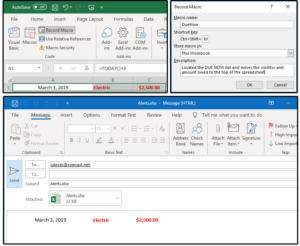 JD Sartain / IDG Worldwide
 Record the macro instruction and email the spreadsheet.
Test your macro
1. Press Ctrl+ Transfer- M. (Press the Ctrl key and hold, insistency the Shift key and hold, press the letter M, and then sackin all three keys at the same time.)
2. The macro runs in a second, then opens Outlook for you to enter the email information.
3. And, once again, after you click Ship, you'rhenium returned to the open Surpass spreadsheet.
Save the spreadsheet as a macro spreadsheet, such atomic number 3Alerts.xlsm, and exit.

Source: https://www.pcworld.com/article/403377/create-excel-alerts-then-write-a-macro-to-email-them.html
Posted by: powerhinglew.blogspot.com
0 Response to "Create Excel Alerts, then write a macro to email them - powerhinglew"
Post a Comment